A Journey Through Statistical Mechanics

"When we gaze at a glass of still water, we see the 'tranquility' and 'certainty' of the macroscopic world. Yet, at the microscopic level, a chaotic storm involving $10^{23}$ actors is unfolding: particles collide, energy fluctuates, and chaos seems inevitable. While classical physics usually seeks precise trajectories, thermal physics teaches us a different kind of wisdom: since we cannot track the dance steps of every single particle, we turn instead to listening to the rhythm of the entire ensemble.

Among the many branches of physics, statistical mechanics possesses a unique logical beauty. It requires neither the intricate force analysis of classical mechanics nor the complex interaction terms of quantum field theory. It requires only one extremely simple axiom—the 'Fundamental Assumption of Statistical Mechanics.' As long as you acknowledge that in an isolated system, every possible microstate appears with equal probability, the rest of the thermodynamic universe—from the definition of temperature to the Boltzmann distribution, from the derivation of chemical potential to Bose-Einstein condensation—can be deduced as naturally as falling dominoes.

This is a story about 'More is Different.' This article aims to strip away complex specific models and restore the original skeleton of thermal physics. We will start from the Multiplicity Function and, guided by Entropy, retrace the marvelous journey from microscopic counting to macroscopic prediction."

Note: This article assumes the reader possesses basic knowledge and concepts of quantum mechanics, as statistical mechanics is inherently quantum in nature. We are, in effect, calculating the statistical effects of massive quantities of quanta.

image 1.png

Chapter 1: The Art of Counting — From Multiplicity to Thermal Equilibrium

Our journey begins with a question so simple it seems outrageous: Under given macroscopic conditions, how many possible microscopic 'ways of living' does a system have?

Physicists have given this number of 'ways' a name: Multiplicity, usually denoted by the symbol $g$ .

1. The Fundamental Assumption: Nature is Fair

Imagine an isolated box containing $N$ particles, with total energy $U$ and volume $V$ . These particles are colliding and moving frantically. At this moment, particle A might be on the left and particle B on the right; the next moment, they might swap positions.

Statistical mechanics is built upon a single, foundational axiom—the Fundamental Assumption:

For an isolated system, all accessible quantum states that satisfy energy conservation appear with equal probability.

This means Nature plays no favorites. As long as the energy allows it, the chance of the system being in state A is exactly the same as being in state B.

2. Why Define Entropy? ( $S = \ln g$ )

If multiplicity $g$ already describes the number of system states, why do we need the concept of "entropy"?

This is not for mystification, but for two extremely pragmatic reasons:

The numbers are too large:
For macroscopic objects, $g$ is an astronomical figure. Even for a small vial of gas, the order of magnitude of $g$ might be $10^{10^{23}}$ . Handling such numbers is not only troublesome but mathematically unintuitive.
We need Additivity:
Imagine you have two glasses of water, System A and System B.
- If you view them as a whole, the total number of states is the product of their individual states: $g_{t o t a l} = g_{A} \times g_{B}$ (combinatorial principle).
- However, in macroscopic physics, we are used to "addition." Mass adds up, volume adds up, energy adds up. We want this quantity describing the "degree of disorder" to be additive as well.

What mathematical tool turns multiplication into addition while taming massive exponents into manageable numbers? The answer is the logarithm.

Thus, Boltzmann (and Planck) provided one of the most profound definitions in physics—Fundamental Entropy:

σ = \ln g

Entropy, in essence, is the logarithm of the number of microstates. It is not some mysterious destructive force; it is simply our measure of a system's "possibility."

3. Why Does Thermal Equilibrium Mean Maximum Entropy?

Now, let us witness the moment of magic.

Suppose we place two independent systems, A and B, together and allow them to make Thermal Contact. This means they can exchange energy, but the total energy $U_{t o t a l} = U_{A} + U_{B}$ remains constant.

How will the system evolve?

According to the Fundamental Assumption, the system will random walk, trying various energy distributions. However, there is one distribution whose probability will overwhelmingly dominate all others—the one that maximizes the total number of microstates $g_{t o t a l}$ .

Mathematically, maximizing $g_{t o t a l}$ is equivalent to maximizing $\ln g_{t o t a l}$ :

\ln g_{t o t a l} = \ln (g_{A} \times g_{B}) = \ln g_{A} + \ln g_{B} = σ_{A} + σ_{B} = σ_{t o t a l}

Using only the single basic assumption of statistical mechanics, the multiplicity of the entire system is $g (U) = \sum_{U_{1}} g_{1} (U_{1}) g_{2} (U - U_{1}) \geq g_{1} (U_{10}) g_{2} (U - U_{10})$ , where $U_{10}$ is the initial energy of subsystem 1. Thus, $\log g (U) \geq \log g_{1} (U_{10}) g_{2} (U_{20})$ , which means $S \geq S_{10} + S_{20}$ . Therefore, entropy increases after thermal contact, essentially proving that the Second Law of Thermodynamics is entirely correct.

Now, if we consider that only the most probable configuration contributes to $g (U)$ , i.e., $g (U) \approx g_{1} ({\hat{U}}_{1}) g_{2} ({\hat{U}}_{2})$ , then according to $\log g (U) \geq \log g_{1} (U_{10}) g_{2} (U_{20})$ , we have ${\hat{S}}_{1} + {\hat{S}}_{2} \geq {\hat{S}}_{10} + {\hat{S}}_{20}$ . This yields a weaker form of the Second Law, often the one learned in introductory courses. However, this form is not entirely rigorous because, after thermal contact, we cannot strictly distinguish between ${\hat{S}}_{1}$ and ${\hat{S}}_{2}$ . We can only say that when thermal contact is weak and heat exchange is not violent, the two subsystems relatively retain their "subjectivity," making this form correct. While this narrative is slightly blurred, it holds true for macroscopic systems we observe daily, though not absolutely.

Conclusion: The system evolves toward thermal equilibrium because that equilibrium state possesses the greatest number of microstates. Entropy increase is, fundamentally, the system evolving in the direction of "more possibilities."

4. The Birth of Temperature: Why Define it as a Derivative?

When two systems reach thermal equilibrium (maximum entropy), what happens? According to calculus, when a function reaches an extremum, its derivative is zero.

We differentiate the total entropy with respect to the energy distribution:

\frac{d σ_{t o t a l}}{d U_{A}} = \frac{\partial σ_{A}}{\partial U_{A}} + \frac{\partial σ_{B}}{\partial U_{A}} = 0

Since energy is conserved ( $d U_{B} = - d U_{A}$ ), we have $\frac{\partial σ_{B}}{\partial U_{A}} = \frac{\partial σ_{B}}{\partial U_{B}} \frac{d U_{B}}{d U_{A}} = - \frac{\partial σ_{B}}{\partial U_{B}}$ .

Substituting this back, we obtain the critically important equilibrium condition:

(\frac{\partial σ_{A}}{\partial U_{A}}) = (\frac{\partial σ_{B}}{\partial U_{B}})

Pause to reflect:

When two objects reach thermal equilibrium, what physical quantity is equal? Intuition tells us it is Temperature.

This implies that the mathematical quantity $\frac{\partial σ}{\partial U}$ must have a profound connection with temperature. Why not define it directly as temperature?

Let's look at the physical meaning of this quantity: it is the "rate of change of entropy with respect to energy."

When you give a cold object a little energy, its disorder (number of states) increases drastically. A cold object is "hungry" for energy ( $\frac{\partial σ}{\partial U}$ is large).
When you give a hot object a little energy, the increase in its disorder is negligible. A hot object is "indifferent" to energy ( $\frac{\partial σ}{\partial U}$ is small).

Since a larger $\frac{\partial σ}{\partial U}$ corresponds to a "colder" object, this is inverse to our habitual definition of temperature (where a higher value means hotter).

Therefore, to align with human cognitive habits, we define the fundamental temperature ( $τ$ ) as the inverse of this quantity:

\frac{1}{τ} \equiv {(\frac{\partial σ}{\partial U})}_{N, V}

This is the rigorous definition of temperature in statistical mechanics: Temperature measures the system's willingness to "pay" energy in exchange for increased entropy.

Low Temperature means a huge entropy gain for a tiny energy cost (high cost-performance ratio).
High Temperature means even a large energy input yields minimal entropy increase.

If examined closely, one finds that the definition of temperature shares the same form as half-life; just as half-life shares dimensions with time, temperature shares dimensions with energy (in natural units).

Chapter 2: The Birth of Pressure

1. Why is Entropy a Function of $U, V, N$ ?

First, we must answer a meta-question: Why do we always write entropy as $σ (U, V, N)$ ?

This is because, at the microscopic level, Multiplicity ( $g$ ), the number of microstates, depends entirely on the "boundary conditions" of the system:

$U$ (Energy): Determines the "budget" you can allocate for particle motion.
$V$ (Volume): Determines the "space" available for particles to occupy (in quantum mechanics, volume determines the wavelength of standing waves, i.e., the energy level structure).
$N$ (Particle Number): Determines how many "actors" are participating in this chaotic performance.

Since $g$ depends on $U, V, N$ , entropy $σ$ , as the logarithm of $g$ , is naturally a function of these three variables.

Previously, we only took the partial derivative with respect to $U$ to define temperature. Now, if we take partial derivatives with respect to $V$ and $N$ , two other core physical quantities will naturally "emerge." In this section, we derive the quantity related to $V$ : pressure.

2. Pressure: The Craving for Spatial Expansion

Imagine replacing our rigid container with a cylinder equipped with a piston. Now, the volume $V$ can change.

When volume changes, quantum mechanics tells us that energy levels actually shift: $E_{s} (V - Δ V) \approx E_{s} (V) - \frac{\partial E_{s}}{\partial V} Δ V$ . With $E_{s} = \frac{π^{2} ℏ^{2}}{2 m L^{2}} (n_{x}^{2} + n_{y}^{2} + n_{z}^{2}) \sim V^{- 2 / 3}$ , as volume decreases, energy levels rise. However, the levels do not cross; this relies on slow compression, technically called an adiabatic process. In such a process, from the perspective of quantum statistics, the distribution of system states remains unchanged. If the system occupied $Ω = 1000$ microstates initially, it still occupies those 1000 microstates after slow compression. Since the number of microstates $Ω$ is unchanged, entropy is invariant. Thus, we can more accurately write: $E_{s} (V - Δ V) \approx E_{s} (V) - (\frac{\partial E_{s}}{\partial V})_{σ} Δ V$ , meaning entropy $σ$ is fixed.

Considering statistical mechanics, we calculate the statistical average: $\sum_{s} P (E_{s}) E_{s} (V - Δ V) = \sum_{s} P (E_{s}) E_{s} (V) - P (E_{s}) (\frac{\partial E_{s}}{\partial V})_{σ} Δ V$ . Since $U = \sum_{s} P (s) E_{s}$ , we have $U (V - Δ V) = U (V) - (\frac{\partial U}{\partial V})_{σ} Δ V$ .
From another angle, the change in energy is the work done by pressure: $Δ U = p Δ V$ .
Thus, we obtain $p = - (\frac{\partial U}{\partial V})_{σ}$ . The negative sign exists because pressure doing positive work causes volume to decrease.

There is another non-trivial way to write Pressure: $p = τ (\frac{\partial σ}{\partial V})_{U}$ . The physics of this is harder to grasp—how can one guarantee $U$ is fixed? However, the mathematical derivation is simple. For a binary function $f (x, y) = C$ , the formula holds: $(\frac{\partial y}{\partial x})_{f} = - (\frac{\partial f}{\partial x})_{y} / (\frac{\partial f}{\partial y})_{x}$ . Letting $f \to σ, x \to V, y \to U$ , we get $(\frac{\partial U}{\partial V})_{σ} = - (\frac{\partial σ}{\partial V})_{U} / (\frac{\partial σ}{\partial U})_{V}$ , which implies $\frac{p}{τ} = (\frac{\partial σ}{\partial V})_{U}$ .

Essentially, pressure represents the intensity of the "desire to expand volume to increase entropy." After all, when volume increases slightly ( $Δ V > 0$ ), the particles' play area expands, and energy levels become denser. Obviously, the number of microstates $g$ increases, and entropy $σ$ increases. Pressure $P$ is a mechanical force pushing against the piston, but here, the driving force is Entropy. $\frac{\partial σ}{\partial V}$ tells us how much disorder you gain per unit of added volume. If the temperature $τ$ is very high, the system is already very chaotic, so the marginal utility of extra disorder from volume is less obvious. Therefore, to maintain the same rate of entropy increase, you need immense pressure.

Chapter 3: A Shift in Perspective — Why Introduce Free Energy?

We already have entropy $σ (U, V, N)$ , and theoretically, we can solve all problems. But in practical operations (or experiments), there is a massive pain point:

It is very difficult to control the total energy $U$ of a system.

Imagine boiling a cup of water in a lab. It is easy to control temperature (using a constant-temperature hot plate) and volume (using a rigid cup), but it is incredibly hard to precisely control how many Joules of internal energy are in that water, as heat flows in and out constantly.

When we switch from an "isolated system" (fixed $U$ ) to a "system in contact with a heat reservoir" (fixed $τ$ ), the original "Maximum Entropy Principle" becomes unwieldy (because due to heat exchange, it is the System Entropy + Environment Entropy that is maximized, not just the system's).

We need a new guiding light—a quantity that tends toward an extremum under fixed temperature $τ$ .

1. Helmholtz Free Energy

Suppose two systems are in thermal contact. One is a massive Heat Reservoir, and the other is the System of interest (fixed $V$ ).

Defining $F = U - τ σ$ , we want to prove that after reaching thermal equilibrium (temperature fixed; reservoir temperature $τ$ , system temperature $τ_{S}$ ), Free Energy becomes a minimum.

Since temperatures are equal at equilibrium, $τ_{S} = (\frac{\partial U_{S}}{\partial σ_{S}})_{V} = τ$ , so $d U_{S} = τ d σ_{S}$ , leading to $d F_{S} = 0$ . This is why we define $F = U - τ σ$ this way—to find an extremum. Recall that for a system and a reservoir, the equilibrium condition is maximizing $σ_{1} + σ_{2}$ . We don't actually care about the reservoir, and minimizing system Free Energy $F$ gives us a way to ignore the reservoir while still determining equilibrium. Let's prove it is a minimum.
Total entropy is $σ = σ_{S} + σ_{R} = σ_{S} (U_{S}) + σ_{R} (U - U_{S})$ . Since the reservoir is huge, we Taylor expand: $\approx σ_{S} (U_{S}) + σ_{R} (U) + (\frac{\partial σ_{R}}{\partial U_{R}})_{V} (- U_{S}) = σ_{R} (U) - U_{S} / τ + σ_{S} = σ_{R} (U) - F_{S} / τ$ . Clearly, maximizing entropy is equivalent to minimizing Free Energy. Note that entropy belongs to the system plus reservoir, but free energy belongs only to the system.
$σ = const - \frac{1}{τ} F_{S}$ . This is a beautiful result. With free energy, we can disregard the reservoir. The reservoir contributes only a $τ$ , which is a fixed constant at equilibrium.

2. Chemical Potential: The Driving Force of Particle Flow

Now we release the final variable: particle number $N$ . We consider a system that can exchange not just energy, but also particles. For example, two systems placed on a reservoir at temperature $τ$ , connected by a small tube for particle exchange. After some time, they reach diffusive equilibrium. (Note: previously we discussed thermal equilibrium $τ_{1} = τ_{2} = τ$ ). In describing this process, we derive the concept of chemical potential.

Crucially, $Δ N_{1} = - Δ N_{2}$ .
Recalling that free energy $F$ must be minimized ( $d F = 0$ ), we have $\frac{\partial F}{\partial N_{1}} d N_{1} + \frac{\partial F}{\partial N_{2}} d N_{2} = 0$ , implying ${(\frac{\partial F}{\partial N_{1}})}_{V, τ} = {(\frac{\partial F}{\partial N_{2}})}_{V, τ}$ .

We introduce the Weak Link Assumption: Assume the tube is thin enough that the two systems are statistically independent (so $F \approx F_{1} + F_{2} = U_{1} + U_{2} - τ (σ_{1} + σ_{2})$ ), but wide enough to allow particle exchange.

Thus, ${(\frac{\partial F_{1}}{\partial N_{1}})}_{V, τ} = {(\frac{\partial F_{2}}{\partial N_{2}})}_{V, τ}$ . This is the equilibrium condition.
From this, we define chemical potential: $μ_{1} = {(\frac{\partial F_{1}}{\partial N_{1}})}_{V, τ} = {(\frac{\partial F_{2}}{\partial N_{2}})}_{V, τ} = μ_{2}$ .

You might ask if a single system needs a chemical potential, since the definition seems to require two. In fact, we can draw an analogy with temperature:

An isolated closed system needs neither $τ$ nor $μ$ . This is the microcanonical ensemble.
If this system contacts a heat reservoir, we need $τ$ but not $μ$ to describe it. This is the canonical ensemble (most common in traditional thermal physics).
If this system contacts a particle reservoir, we don't need $τ$ but need $μ$ . While such systems exist (where particles are "virtual," carrying no energy, like information), they are rare in standard material physics.
If the system contacts both a heat and particle reservoir, we need both $τ$ and $μ$ . This is the grand canonical ensemble.

Previously, the definition of pressure was derived from energy $U$ , but we found it could be transformed into the partial derivative of entropy $σ$ with respect to volume $V$ . Now, having defined chemical potential from free energy $F$ , we discover a link to the partial derivative of entropy $σ$ with respect to particle number $N$ . We need two calculus formulas: $\frac{d y}{d x} = \frac{1}{\frac{d x}{d y}}$ and $\frac{d y}{d x} = - \frac{\frac{\partial f}{\partial x}}{\frac{\partial f}{\partial y}}$ .

Using the first, we directly get ${(\frac{\partial U}{\partial σ})}_{N, V} = \frac{1}{{(\frac{\partial σ}{\partial U})}_{N, V}}$ .

Using the second, we get ${(\frac{\partial σ}{\partial N})}_{U, V} = - \frac{{(\frac{\partial U}{\partial N})}_{σ V}}{{(\frac{\partial U}{\partial σ})}_{V, N}} = - \frac{μ}{τ}$ .

Chemical potential describes the system's willingness to "accept new particles to increase entropy." The physical intuition is that matter tends to flow from high to low (water flows down, charge flows to low potential). Here, particles naturally flow from High Chemical Potential to Low Chemical Potential (to maximize total entropy). Without the negative sign, particles would counter-intuitively flow from low to high.

Chapter 4: Thermodynamic Identities — Different Faces of the Same Truth

We have defined entropy, temperature, pressure, and chemical potential. Now, we enter the interior of the edifice to explore the intricate yet symmetrical relationships between these quantities. Through the art of differentiation, we will reveal the essence of the First Law of Thermodynamics and show how to navigate different "energy landscapes" via mathematical transformations. You will find that thermal physics, unlike classical mechanics with its single core law ( $F = m a$ ), seems to possess countless faces—internal energy, enthalpy, free energy, Gibbs energy... But do not get lost; these faces are merely projections of the same truth under different lighting.

1. Three Ways to Write the First Law

Let's play a differential game to see what results from starting with different functions.

Perspective 1: Entropy $σ (U, V)$

If we view entropy as a function of internal energy and volume, its total differential is:

d σ = {(\frac{\partial σ}{\partial U})}_{V} d U + {(\frac{\partial σ}{\partial V})}_{U} d V

Recall our definitions: $\frac{1}{τ} = (\frac{\partial σ}{\partial U})_{V}$ and $\frac{P}{τ} = (\frac{\partial σ}{\partial V})_{U}$ . Substituting these:

d σ = \frac{1}{τ} d U + \frac{P}{τ} d V

Multiplying by $τ$ :

τ d σ = d U + P d V

Or the familiar form: $d U = τ d σ - P d V$ .

Here $τ d σ$ corresponds to heat $d Q$ , and $- P d V$ to work $d W$ .

Conclusion: The First Law of Thermodynamics (Energy Conservation) is mathematically equivalent to the fact that "entropy is a function of state variables $U$ and $V$ ."

Perspective 2: Internal Energy $U (σ, V)$

If we flip the perspective and view internal energy as a function of entropy and volume:

d U = {(\frac{\partial U}{\partial σ})}_{V} d σ + {(\frac{\partial U}{\partial V})}_{σ} d V = τ d σ - p d V

This is still the First Law, but the viewpoint has shifted: Temperature is the slope of internal energy vs. entropy, and Pressure is the slope of internal energy vs. volume.

Perspective 3: Free Energy $F (τ, V)$

This is the most brilliant step. Recall $F = U - τ σ$ . Differentiating:

d F = d U - d (τ σ) = d U - σ d τ - τ d σ

Substituting $d U = τ d σ - P d V$ :

d F = (τ d σ - P d V) - σ d τ - τ d σ

The term $τ d σ$ cancels perfectly! We are left with:

d F = - P d V - σ d τ

This means if we view $F$ as a function of $τ$ and $V$ , its total differential $d F = {(\frac{\partial F}{\partial τ})}_{V} d τ + {(\frac{\partial F}{\partial V})}_{τ} d V$ tells us:

{(\frac{\partial F}{\partial τ})}_{V} = - σ, {(\frac{\partial F}{\partial V})}_{τ} = - P

2. The Core Truth: $d σ = 0$

Faced with so many formulas, you might ask: What is the core of thermal physics? Is there a governing formula like $F = m a$ ?

The answer is yes. The soul of thermal physics is $d σ = 0$ .

Let's prove this with a thought experiment. Consider two systems $S_{1}$ and $S_{2}$ in thermal contact. We allow the most thorough exchange:

Energy Exchange: $U_{1} + U_{2} = U_{c o n s t}$
Volume Exchange (Movable partition): $V_{1} + V_{2} = V_{c o n s t}$
Particle Exchange (Perforated partition): $N_{1} + N_{2} = N_{c o n s t}$

When does the system reach equilibrium? When total entropy is maximized, i.e., $d σ = 0$ .

Approximating $σ \approx σ_{1} + σ_{2}$ :

d σ = d σ_{1} + d σ_{2} = 0

Expanding the differentials:

[\frac{\partial σ_{1}}{\partial U_{1}} d U_{1} + \frac{\partial σ_{1}}{\partial V_{1}} d V_{1} + \frac{\partial σ_{1}}{\partial N_{1}} d N_{1}] + [\frac{\partial σ_{2}}{\partial U_{2}} d U_{2} + \frac{\partial σ_{2}}{\partial V_{2}} d V_{2} + \frac{\partial σ_{2}}{\partial N_{2}} d N_{2}] = 0

Using conservation relations $d U_{2} = - d U_{1}$ , etc., and grouping terms:

(\frac{\partial σ_{1}}{\partial U_{1}} - \frac{\partial σ_{2}}{\partial U_{2}}) d U_{1} + (\frac{\partial σ_{1}}{\partial V_{1}} - \frac{\partial σ_{2}}{\partial V_{2}}) d V_{1} + (\frac{\partial σ_{1}}{\partial N_{1}} - \frac{\partial σ_{2}}{\partial N_{2}}) d N_{1} = 0

Since $U, V, N$ are independent, for the equation to hold, the terms in brackets must be zero. This leads directly to all equilibrium conditions:

Energy Equilibrium: $\frac{1}{τ_{1}} = \frac{1}{τ_{2}}$ (Equal Temperature)
Volume Equilibrium: $\frac{P_{1}}{τ_{1}} = \frac{P_{2}}{τ_{2}}$
Particle Equilibrium: $- \frac{μ_{1}}{τ_{1}} = - \frac{μ_{2}}{τ_{2}}$

Key Insight: Strictly speaking, the conditions for equilibrium are the equality of $P / τ$ and $μ / τ$ . It is only because we typically also exchange energy (making $τ$ equal) that we get the familiar $P_{1} = P_{2}$ and $μ_{1} = μ_{2}$ . All thermodynamic quantities essentially emerge from the extremum condition $d σ = 0$ .

3. Conjugate Variables — Dancing Partners

If we look back at internal energy $U (σ, V, N)$ , we see a pattern.

The independent variables $σ, V, N$ are all Extensive Variables (scaling with system size). Internal energy $U$ is also extensive.

Physicists define Generalized Force:

f_{i} = \frac{\partial U}{\partial x_{i}}

This reveals that physical quantities appear in pairs, each containing one extensive and one intensive quantity, known as Conjugate Variables:

Extensive Variable	Intensive Variable / Generalized Force	Physical Meaning
Entropy $σ$	Temperature $τ$	$(\partial U / \partial σ)_{V, N}$
Volume $V$	Pressure $- P$	$(\partial U / \partial V)_{σ, N}$
Particle Number $N$	Chemical Potential $μ$	$(\partial U / \partial N)_{σ, V}$

This offers a new perspective to understand thermal physics via classical mechanics (force balance): Thermal equilibrium is essentially the static equilibrium of generalized forces.

4. Legendre Transformation — Changing the Subject

Finally, we explain mathematically why the construction $F = U - τ σ$ is so important.

In experiments, controlling entropy $σ$ is extremely hard, but controlling temperature $τ$ is simple. We want to transform the system description from $U (σ, \dots)$ to $F (τ, \dots)$ . This transformation is called a Legendre Transformation.

Consider a function $U (σ)$ with slope $τ = \frac{d U}{d σ}$ . If we define:

F (τ) \equiv U (σ) - τ σ

(Note: here $σ$ and $τ$ are not independent; $σ$ is a function of $τ$ ).

Differentiation gives:

\frac{d F}{d τ} = \frac{d}{d τ} (U - τ σ) = \frac{d U}{d σ} \frac{d σ}{d τ} - σ - τ \frac{d σ}{d τ}

Since $\frac{d U}{d σ} = τ$ , the first and third terms cancel, leaving:

\frac{d F}{d τ} = - σ

This is the magic of Duality: it changes the independent variable from $σ$ to $τ$ , while the original variable $σ$ becomes the derivative of the new function (with a negative sign).

This holds for multivariate functions $F (τ, V, N) = U (σ, V, N) - τ σ$ , preserving other partial derivatives:

${(\frac{\partial F}{\partial τ})}_{N, V} = - σ$ (New)
${(\frac{\partial F}{\partial V})}_{τ, N} = {(\frac{\partial U}{\partial V})}_{σ, N} = - P$ (Unchanged)
${(\frac{\partial F}{\partial N})}_{τ, V} = {(\frac{\partial U}{\partial N})}_{σ, V} = μ$ (Unchanged)

We have now derived all thermodynamic relations and understood why Free Energy acts as a potential function tailored for a reality where "temperature is easier to control than entropy."

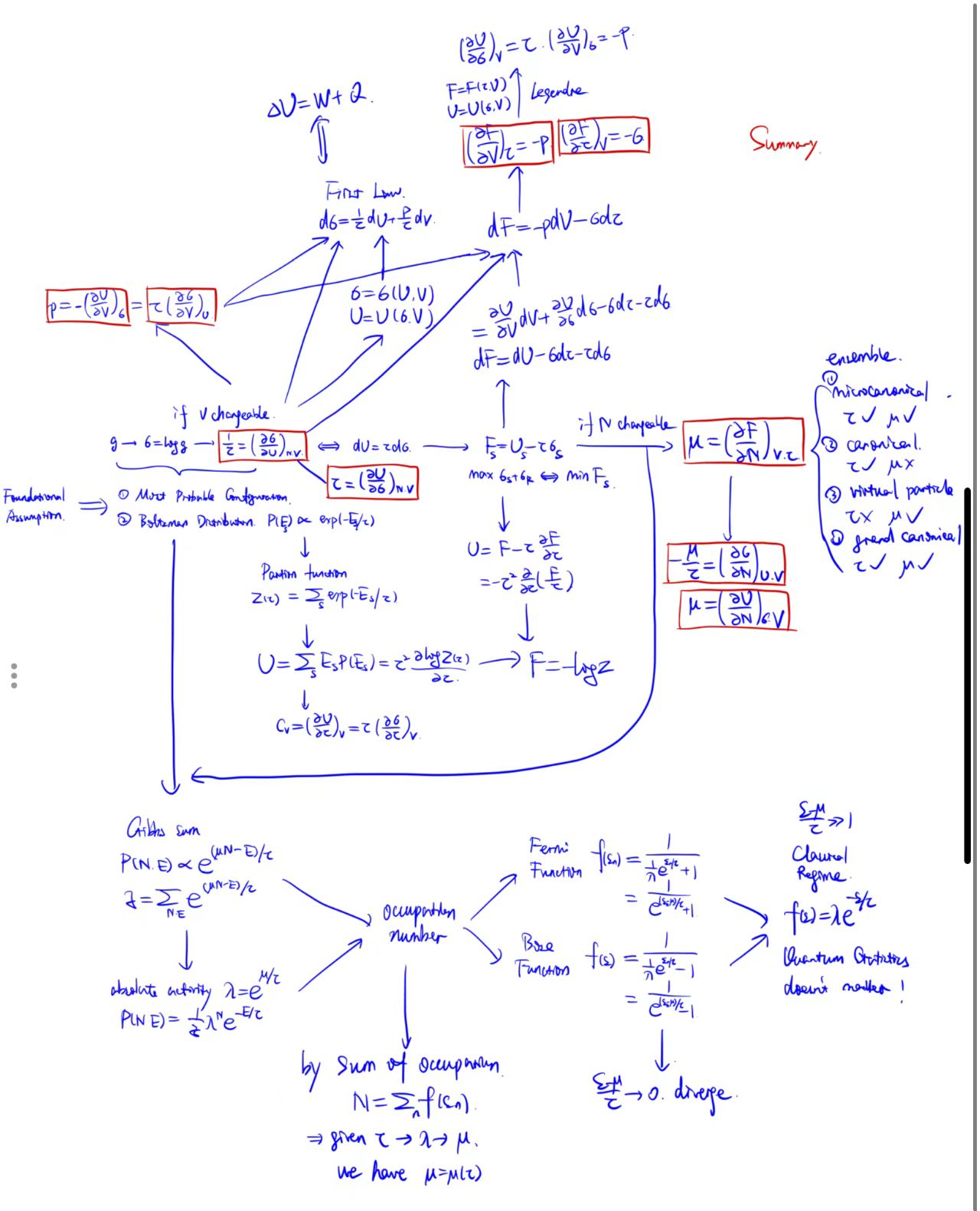
Chapter 5: The Rosetta Stone of Thermal Physics

After four chapters, we have examined the system from three angles: Microscopic Counting (Entropy), Energy Conservation (Internal Energy), and Pragmatism (Free Energy). It seems like the blind men and the elephant—different parts, different descriptions. If we align the three potentials $σ, U, F$ and examine their partial derivatives, we get this symmetrical table:

Quantity	Entropy Representation σ(U,V,N)	Internal Energy Representation U(σ,V,N)	Free Energy Representation F(τ,V,N)
Temp $τ$	$\frac{1}{τ} = {(\frac{\partial σ}{\partial U})}_{V, N}$	$τ = {(\frac{\partial U}{\partial σ})}_{V, N}$	$σ = - {(\frac{\partial F}{\partial τ})}_{N, V}$
Pressure $P$	$\frac{P}{τ} = {(\frac{\partial σ}{\partial V})}_{U, N}$	$- P = {(\frac{\partial U}{\partial V})}_{σ, N}$	$- P = {(\frac{\partial F}{\partial V})}_{τ, N}$
Chem Pot $μ$	$- \frac{μ}{τ} = {(\frac{\partial σ}{\partial N})}_{U, V}$	$μ = {(\frac{\partial U}{\partial N})}_{σ, V}$	$μ = {(\frac{\partial F}{\partial N})}_{τ, V}$

We must interpret three layers of information from this table.

1. The "Definitions" on the Diagonal

While every equation is mathematically valid, physicists typically use the diagonal from top-left to bottom-right to establish definitions:

Row 1, Col 1: $\frac{1}{τ} = \frac{\partial σ}{\partial U}$ . The Statistical Mechanics Definition of temperature.
Row 2, Col 2: $- P = \frac{\partial U}{\partial V}$ . The Mechanical Definition of pressure (Generalized Force).
Row 3, Col 3: $μ = \frac{\partial F}{\partial N}$ . The Practical Definition of chemical potential (change in free energy when adding a particle at constant $T$ ).

2. "The One Truth" and Redundancy

Do you need to memorize all 9 formulas? No.

The last two columns are technically "redundant." The entire physics is contained in the first column (Entropy).

Once you have $σ = σ (U, V, N)$ , you have the universe.
Column 2 ( $U$ ) is just an inverse function.
Column 3 ( $F$ ) is just a Legendre transform.

Physicists keep them not for new information, but for coordinate convenience (it is easier to hold $τ$ constant than $σ$ ).

3. Mathematical Bridges

How do you derive Column 2 from Column 1? It's just calculus.

Bridge 1: Reciprocal Relation

Comparing Row 1: $\frac{1}{τ} = (\frac{\partial σ}{\partial U})$ vs $τ = (\frac{\partial U}{\partial σ})$ .

This uses the Inverse Function Rule: $\frac{d y}{d x} = \frac{1}{\frac{d x}{d y}}$ . This proves the equivalence of the temperature definitions.

Bridge 2: Cyclic Relation

Comparing Row 3: $- \frac{μ}{τ} = (\frac{\partial σ}{\partial N})_{U}$ vs $μ = (\frac{\partial U}{\partial N})_{σ}$ .

Why the strange $- \frac{μ}{τ}$ ? This uses the Triple Product Rule:

{(\frac{\partial y}{\partial x})}_{z} = - \frac{{(\frac{\partial z}{\partial x})}_{y}}{{(\frac{\partial z}{\partial y})}_{x}}

Letting $y = σ, x = N, z = U$ :

{(\frac{\partial σ}{\partial N})}_{U} = - \frac{{(\frac{\partial U}{\partial N})}_{σ}}{{(\frac{\partial U}{\partial σ})}_{N}}

Substituting definitions from Column 2 (numerator is $μ$ , denominator is $τ$ ), we get ${(\frac{\partial σ}{\partial N})}_{U} = - \frac{μ}{τ}$ . The negative sign and division by $τ$ are mathematical necessities, not new physical laws.

Chapter 6: The Great Reversal — From Partition Functions to Gibbs Sums

We spent chapters building thermodynamics from microscopic counting ( $g$ ). But in practice, Conceptual Logic and Computational Logic are often opposites.

Concept: $g \to σ \to τ \to Equilibrium$ .
Computation: $g$ is usually despairingly hard to calculate (imagine counting permutations of $10^{23}$ particles).

So, physicists invented a "Reverse Channel": Write the energy model, calculate the Partition Function ( $Z$ ), get Free Energy ( $F$ ), and then derive Entropy ( $σ$ ) and Multiplicity ( $g$ ).

We introduce two superstars: Boltzmann Distribution (fixed $N$ ) and Gibbs Distribution (variable $N$ ). Instead of counting states, we ask: If we throw the system into a giant reservoir, what is the probability of it being in a specific state?

1. Boltzmann Distribution

Consider System $S$ in contact with a huge Reservoir $R$ . They exchange energy and reach equilibrium (same $τ$ ).

Since we specify a precise microstate of $S$ (Multiplicity = 1), the probability depends entirely on how many ways the Reservoir can accommodate the remaining energy.

The probability ratio equals the ratio of the Reservoir's multiplicities:

\frac{P (E_{1})}{P (E_{2})} = \frac{g_{R} (U_{t o t a l} - E_{1})}{g_{R} (U_{t o t a l} - E_{2})}

Using $σ = \ln g$ ( $g = e^{σ}$ ) and Taylor expanding entropy ( $σ_{R} (U - E) \approx σ_{R} (U) - E / τ$ ), the constant terms cancel, yielding the famous Boltzmann Factor:

P (E) \propto e^{- E / τ}

Information Entropy Perspective:

If we seek the "most unbiased" probability distribution (maximizing Shannon Entropy $σ_{I} = - \sum p_{n} \ln p_{n}$ ) given only the average energy $U$ , Lagrange multipliers similarly yield $p_{n} = C e^{- E_{n} / τ}$ . The Boltzmann distribution is Nature's most "natural," unbiased choice.

2. The Partition Function: The Holy Grail

To normalize $P (E_{s}) \propto e^{- E_{s} / τ}$ , we need the Partition Function ( $Z$ ):

Z \equiv \sum_{all states s} e^{- E_{s} / τ}

So $P (s) = \frac{1}{Z} e^{- E_{s} / τ}$ .

Why is it the "Holy Grail"?

Using $P (s) = e^{(F - E_{s}) / τ}$ and summing to 1 ( $e^{F / τ} Z = 1$ ), we get:

F = - τ \ln Z

The Computational U-Turn:

List Microscopic Model (Energy levels $E_{n}$ ).
Sum to find $Z$ (Geometric series or Gaussian integral).
Find $F$ ( $F = - τ \ln Z$ ).
Find Everything ( $σ$ , $P$ , $μ$ , $U$ via derivatives of $F$ ).

3. Gibbs Sum: When Particles Flow

If the system exchanges particles too (Grand Canonical), the Reservoir's entropy $σ_{R}$ changes with both Energy and Particle Number.

Taylor expansion adds a term:

Δ σ_{R} = \frac{1}{τ} (- E) + (- \frac{μ}{τ}) (- N) = \frac{μ N - E}{τ}

This gives the Gibbs Distribution:

P (N, E) \propto e^{(μ N - E) / τ}

The normalization constant is the Grand Partition Function or Gibbs Sum ( $Z$ ):

Z \equiv \sum_{N = 0}^{\infty} \sum_{s (N)} e^{(μ N - E_{s}) / τ}

Defining Absolute Activity $λ \equiv e^{μ / τ}$ :

P (N, E) = \frac{1}{Z} λ^{N} e^{- E / τ}

A Paradox? In Boltzmann, $e^{- E / τ}$ implies higher energy means lower probability. In Gibbs, $e^{μ N / τ}$ suggests more particles mean higher probability? Will the system explode? No, because for classical ideal gases, chemical potential is typically a large negative value.

Chapter 7: Quantum Statistics — When Particles Lose Their Names

Finally, we address the elephant in the room—Quantum Mechanics. Previously, we treated particles as distinguishable "balls." Now, we face the reality of Indistinguishability.

1. Who is it? No, What is it?

In the quantum world, identical particles are fundamentally indistinguishable. Exchanging two particles leaves the probability density $| Ψ |^{2}$ unchanged: $Ψ (1, 2) = \pm Ψ (2, 1)$ .

This $\pm$ sign divides the universe:

Bosons (+1): Social, like to cluster (Photons, Helium-4).
Fermions (-1): Anti-social, follow Pauli Exclusion, never occupy the same state (Electrons, Protons).

Counting Changes:

Putting 2 particles in 4 energy levels:

Classical: $4^{2} = 16$ ways.
Bosons: 10 ways (Enhanced probability of being together).
Fermions: 6 ways (Zero probability of being together).
Since $g$ changes, Entropy $σ$ and macro-properties change.

2. From Particle View to Orbital View

Instead of asking "Where is Particle A?", we ask "How many particles are in Energy Level $ε$ ?"

Since the number of particles in a level can vary, we use the Gibbs Sum.

3. Fermi-Dirac and Bose-Einstein Distributions

Fermions:

Occupancy $n$ is 0 or 1.

Z = 1 + λ e^{- ε / τ}

Average occupancy:

⟨ n ⟩ = \frac{1}{e^{(ε - μ) / τ} + 1}

The $+ 1$ in the denominator is the mathematical signature of Fermion "social anxiety."

Bosons:

Occupancy $n$ is $0, 1, \dots \infty$ . Geometric series sum:

Z = \frac{1}{1 - λ e^{- ε / τ}}

Average occupancy:

⟨ n ⟩ = \frac{1}{e^{(ε - μ) / τ} - 1}

The $- 1$ leads to Bose-Einstein Condensation if $ε \approx μ$ .

4. Classical Limit: All Roads Lead to Rome

Why don't we feel this difference daily? Because we live in the Classical Regime: High temperature or low density ( $(ε - μ) / τ ≫ 1$ ).

The $\pm 1$ becomes negligible:

\frac{1}{e^{(ε - μ) / τ} \pm 1} \approx e^{μ / τ} e^{- ε / τ}

This is the Boltzmann Distribution!

However, when we cool down past the Quantum Concentration ( $n_{Q}$ ), miracles happen: Fermions form "Fermi Seas" (supporting White Dwarfs), and Bosons collapse into Superfluids.

Conclusion: Order Emerging from Ignorance

Our journey ends here. Let us look back at the structure we built.

We started with an admission of "ignorance": the Principle of Equal Probability.
We quantified "possibility" via Counting and Entropy.
By maximizing entropy, we discovered macroscopic islands of Temperature, Pressure, and Chemical Potential emerging from the chaotic microscopic sea.
We navigated via Free Energy and used Partition Functions as our compass.
Finally, injecting Quantum nature, the framework predicted states of matter under extreme conditions.

Notably, we barely mentioned specific substances. We didn't calculate the specific heat of copper or the rotation of oxygen. That is the charm of statistical mechanics: It is a universal grammar, not a specific story.

It describes the logic of "Many," not the identity of "One." Whether it's molecules in a gas, photons in a cavity, or nuclear matter in a star, as long as you input the Hamiltonian, the macro-properties emerge automatically.

What is Thermal Physics?

It is the science of "More." It is about how, when countless tiny individuals gather, a new, deterministic macroscopic order emerges through statistical laws—an order not possessed by the individuals themselves.

This is perhaps the deepest poetry in physics: God does not need to play dice; chaos itself is the source of order.