Fundamentals of Quantum Computing

This post summarizes the core concepts of quantum computing, starting from classical reversible gates and moving through the fundamental postulates of quantum states and dynamics.

1. Classical Gates and Reversible Computing

1.1 Universality

A set of gates is called universal if it can compute any function $f:\{0,1{\}}^n\to \{0,1\}$.

• Examples of universal sets include $\{\text{AND},\text{OR},\text{NOT}\},\{\text{AND},\text{NOT}\}$, and the single gate $\{\text{NAND}\}$.

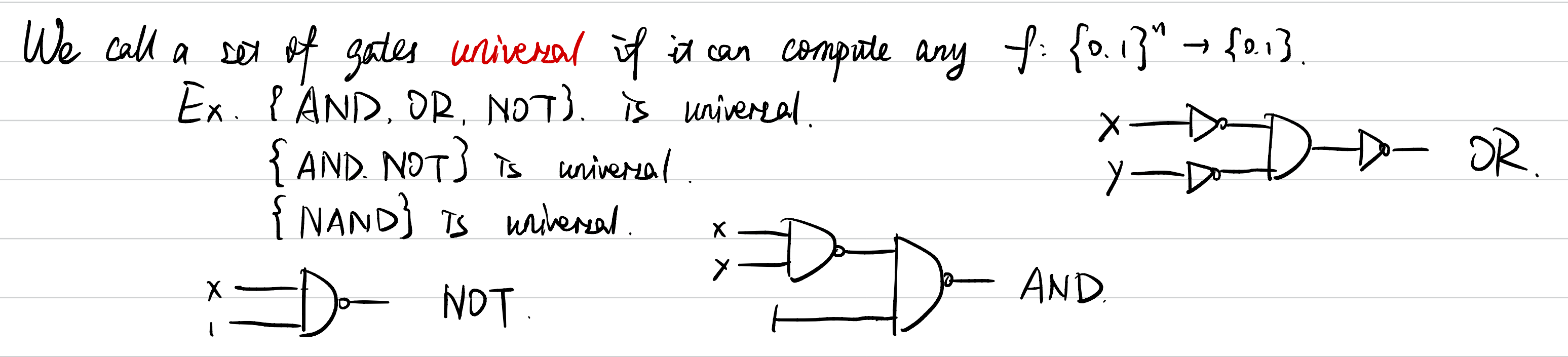
1.2 The Need for Reversibility

Standard classical gates like AND are not reversible because you cannot uniquely determine the inputs $x,y$ from the output $x\cdot y$. In quantum computing, evolution must be reversible.

• The Unitary Nature of Quantum Mechanics: The time evolution of any closed quantum system is described by a Unitary Operator ($U$). In linear algebra, a matrix $U$ is unitary: $U{U}^{†}=I$.
  • Because $U$ has an inverse ($U^{†}$), you can always "undo" the operation.
  • The evolution $U$ is derived from the Schrödinger Equation. When the Hamiltonian ($H$) of a system is time-independent, the evolution is expressed as $e^{-iHt/\hslash }$, which is inherently a unitary (and thus reversible) operator.
  • Unitary transformations preserve the $L_2$-norm (the total probability) of the quantum state, ensuring it remains exactly 1 throughout the evolution.
• Information Conservation: In classical computing, operations like AND are irreversible because they discard information.
  • No Information Loss: In a quantum system, information cannot be "deleted" or "lost" into thin air; it must be preserved within the system's state.
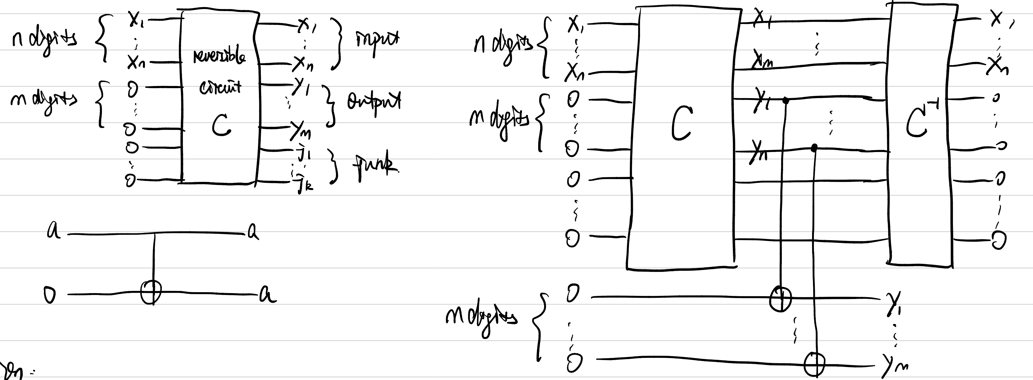
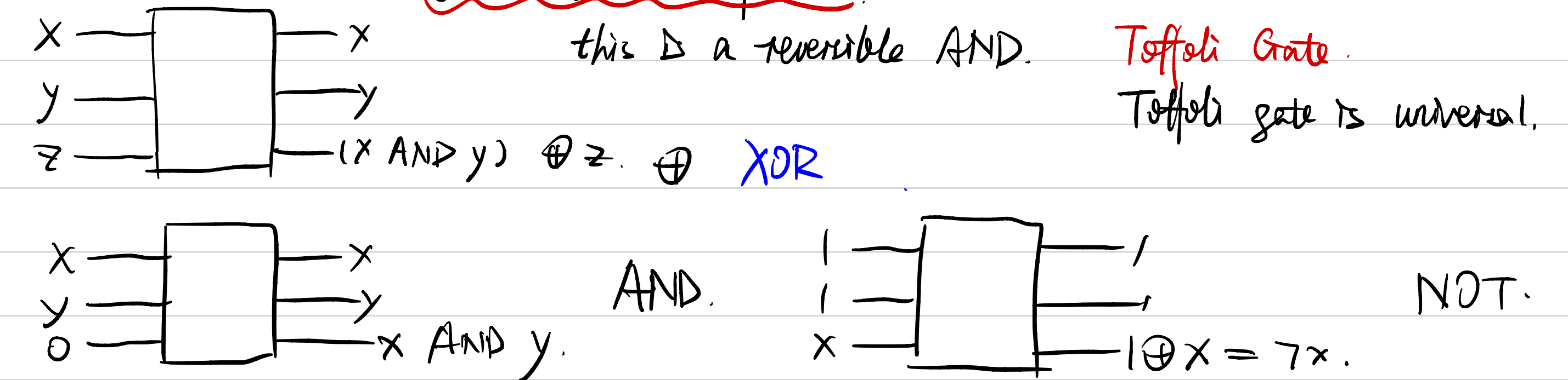
  • The Toffoli Gate Example: To perform classical-style logic (like AND) in a quantum way, we use reversible gates like the Toffoli gate (Controlled-Controlled-NOT) which is also universal. This gate uses an Ancilla bit to store the result while keeping the original inputs intact, allowing the entire process to be reversed.
  • Whenever we can compute $f(x)$ efficiently in polynomial time, we can efficiently compute the reversible mapping $(x,0,0)\mapsto (x,f(x),0)$.

• Physical Heat and Landauer's Principle: the physical reason for pursuing reversibility is often related to energy.
  • Heat Generation: Landauer's Principle states that erasing 1 bit of information releases a specific amount of heat into the environment.
  • Energy Efficiency: Because quantum evolution is unitary (reversible), it theoretically does not require the erasure of information, which is a key requirement for building hardware that avoids the massive heat dissipation seen in classical high-performance chips.

2. Postulates of Quantum Computing: States

2.1 The Qubit

A qubit is represented by a complex vector in a two-dimensional Hilbert space:

where $\alpha ,\beta \in \mathbb{C}$ are amplitudes satisfying the normalization condition $|\alpha {|}^2+|\beta {|}^2=1$.

• Computational Basis: The vectors $|0⟩=(\genfrac{}{}{0ex}{}{1}{0})$ and $|1⟩=(\genfrac{}{}{0ex}{}{0}{1})$ form the standard basis for a qubit.
• Dirac Notation:
  • Ket $|\psi ⟩$: A column vector.
  • Bra $⟨\psi |$: The conjugate transpose (dual vector) of a ket, represented as a row vector.
  • Inner Product: $⟨\psi |\varphi ⟩=a_0^{\ast }{b}_0+a_1^{\ast }{b}_1$.
  • Outer Product: $|0⟩⟨0|+|1⟩⟨1|=I$ (the Identity matrix).

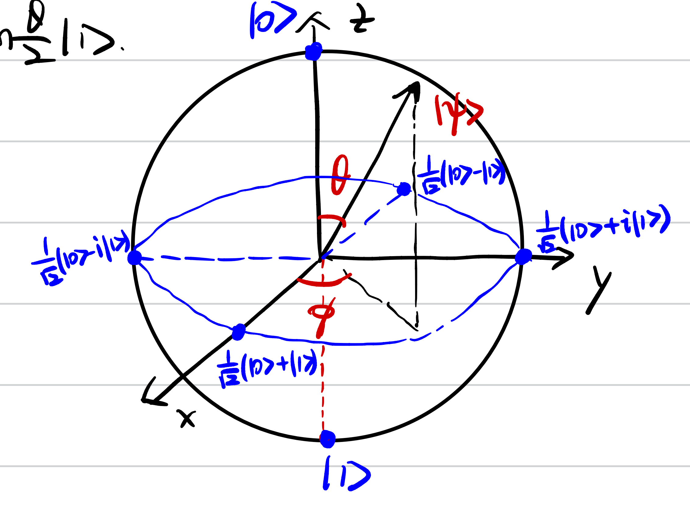
2.2 The Bloch Sphere

Any single-qubit state can be visualized as a point on the Bloch Sphere using the following parameters:

where $\theta$ and $\varphi$ are real numbers defining the point's coordinates.

3. Quantum Dynamics

The time evolution of a closed quantum system is described by a Unitary Transformation.

• A matrix $U$ is unitary if $U{U}^{†}=U^{†}U=I$.
• This ensures that the state remains normalized: $⟨\psi |U^{†}U|\psi ⟩=⟨\psi |\psi ⟩=1$.

Common Single-Qubit Gates

• Pauli Gates: $X=\left(\begin{array}{cc}0& 1\\ 1& 0\end{array}\right)$, $Y=\left(\begin{array}{cc}0& -i\\ i& 0\end{array}\right)$, $Z=\left(\begin{array}{cc}1& 0\\ 0& -1\end{array}\right)$.

• Hadamard (H): $H=\frac{1}{\sqrt{2}}\left(\begin{array}{cc}1& 1\\ 1& -1\end{array}\right)$.

• Phase Gates: $S=\left(\begin{array}{cc}1& 0\\ 0& i\end{array}\right)$ (Note: Corrected from notes) and $T=\left(\begin{array}{cc}1& 0\\ 0& e^{i\pi /4}\end{array}\right)$.

4. Composite Systems and Entanglement

4.1 Tensor Products

The state space of a composite system is the tensor product of its individual component spaces. For example, if we have two qubits in states $|\psi ⟩$ and $|\varphi ⟩$, the combined state is $|\psi ⟩\otimes |\varphi ⟩$ (often written as $|\psi \varphi ⟩$).

4.2 Quantum Entanglement

• Product States: States that can be written in the form $|\psi ⟩\otimes |\varphi ⟩$.
• Entangled States: States that cannot be decomposed into a product of individual qubit states.
  • Example: The state $\frac{1}{\sqrt{2}}(|00⟩+|11⟩)$ is entangled. Proof: Setting ${\alpha }_0{\beta }_1={\alpha }_1{\beta }_0=0$ while ${\alpha }_0{\beta }_0={\alpha }_1{\beta }_1=\frac{1}{\sqrt{2}}$ leads to a contradiction.

Practical Implementation

from qiskit import QuantumCircuit
from qiskit.quantum_info import Statevector

# 1. Create a Bell State (Entangled State)
qc = QuantumCircuit(2)
qc.h(0)     # Apply Hadamard to the first qubit
qc.cx(0, 1) # Apply CNOT (controlled by q0, targeting q1)

# View the statevector
state = Statevector.from_instruction(qc)
print("Bell State Vector:")
print(state.data)

# 2. Apply a gate to a subsystem: (I ⊗ X) acting on the Bell state
qc.x(1) 
final_state = Statevector.from_instruction(qc)
print("\nState after (I ⊗ X):")
print(final_state.data)